Impact of tax credit on single women employment

import numpy as np
import pandas as pd

# pull the data
dataset = pd.read_stata("datasets/eitc.dta")

dataset.head()

	state	year	urate	children	nonwhite	finc	earn	age	ed	work	unearn
0	11.0	1991.0	7.6	0	1	18714.394273	18714.394273	26	10	1	0.000000
1	12.0	1991.0	7.2	1	0	4838.568282	471.365639	22	9	1	4.367203
2	13.0	1991.0	6.4	2	0	8178.193833	0.000000	33	11	0	8.178194
3	14.0	1991.0	9.1	0	1	9369.570485	0.000000	43	11	0	9.369570
4	15.0	1991.0	8.6	3	1	14706.607930	14706.607930	23	7	1	0.000000

Each row is an observation of a single woman.

dataset.shape

(13746, 11)

# creating the modelling dummy variables
dataset['is_mom'] = np.where(dataset['children'] > 0, 1, 0)
dataset['after93'] = np.where(dataset['year'] > 1993, 1, 0)
dataset['is_mom_after93'] = dataset['is_mom'] * dataset['after93']

import matplotlib.pyplot as plt

fig, ax = plt.subplots(figsize=(7,4))

dataset.groupby(['year', 'is_mom'])['work'].mean().unstack().plot(ax=ax)
ax.axvline(1993, color='k', linestyle='--', linewidth=1)
ax.set_xlabel('Year')
ax.set_ylabel('Work rate')
# include a arrow that indicates points from text to the line
ax.annotate('Policy\napplication', 
            xy=(1992.95, 0.5), 
            xytext=(1991.7, 0.53), 
            arrowprops={"width": 3, "headwidth": 10, "color": "orange"});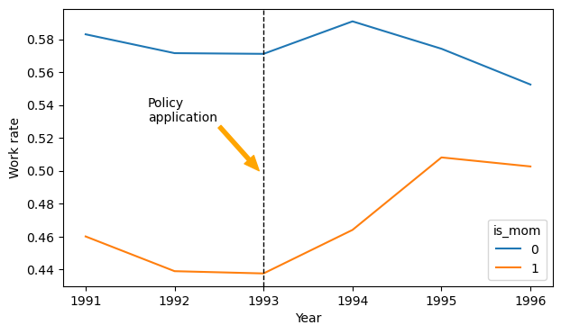

dataset.head()

	state	year	urate	children	nonwhite	finc	earn	age	ed	work	unearn	is_mom
0	11.0	1991.0	7.6	0	1	18714.394273	18714.394273	26	10	1	0.000000	0
1	12.0	1991.0	7.2	1	0	4838.568282	471.365639	22	9	1	4.367203	1
2	13.0	1991.0	6.4	2	0	8178.193833	0.000000	33	11	0	8.178194	1
3	14.0	1991.0	9.1	0	1	9369.570485	0.000000	43	11	0	9.369570	0
4	15.0	1991.0	8.6	3	1	14706.607930	14706.607930	23	7	1	0.000000	1

DiD by aggregation

dataset.groupby(['is_mom', 'after93'])['work'].mean().unstack()

after93	0	1
is_mom
0	0.575460	0.573386
1	0.445962	0.490761

work(is mom after 93) - work(is_mom before 93) = 0.49 - 0.45 = 0.4
work(not mom after 93) - work(not mom before 93) = 0.57 - 0.58 = -0.1
DiD = 0.4 - (-0.1) = 0.4 + 0.1 = 0.5
DiD = 0.5

The employmet rate of mom’s that work has increased by 0.5 after the policy application.

DiD by Logistic Regression

X = dataset[['is_mom', 'after93', 'is_mom_after93']]
y = dataset['work'].values

import statsmodels.api as sm

X = sm.add_constant(X)
model1 = sm.Logit(y, X).fit()

Optimization terminated successfully.
         Current function value: 0.686491
         Iterations 4

print(model1.summary())

                           Logit Regression Results                           
==============================================================================
Dep. Variable:                      y   No. Observations:                13746
Model:                          Logit   Df Residuals:                    13742
Method:                           MLE   Df Model:                            3
Date:                Wed, 28 Dec 2022   Pseudo R-squ.:                0.009118
Time:                        20:39:39   Log-Likelihood:                -9436.5
converged:                       True   LL-Null:                       -9523.3
Covariance Type:            nonrobust   LLR p-value:                 2.058e-37
==================================================================================
                     coef    std err          z      P>|z|      [0.025      0.975]
----------------------------------------------------------------------------------
const              0.3042      0.036      8.443      0.000       0.234       0.375
is_mom            -0.5212      0.047    -10.985      0.000      -0.614      -0.428
after93           -0.0085      0.053     -0.161      0.872      -0.112       0.095
is_mom_after93     0.1885      0.070      2.708      0.007       0.052       0.325
==================================================================================

It is not the same because it is a Logistic Regression!